


In plane geometry, the term tessellation indicates the covering of the plane with one or more geometric figures (called “tiles”) repeated infinitely, without overlapping and without spaces between them.
Similarly, in the origami world, all those models formed by equal (or even similar) “tiles” that are repeated in the surface are called tessellations.
Each tessellation is always made from a single sheet of paper properly folded.
Unlike geometric tessellations, the tessellations can be both flat and three-dimensional.
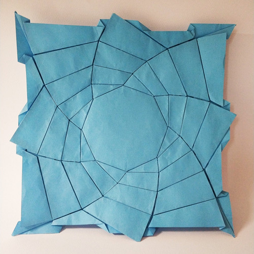
“Flagstone” tessellations
The origami tessellations can be divided into various subgroups, each with its own particular characteristics.
One of these subgroups is that of flagstone tessellations.
These are tessellations in which the edges of the tiles forming them are adjacent and on the same level, without overlapping.
They are reminiscent of flagstone flooring, hence the name “flagstone”.
In the image below there are some examples of these tessellations.
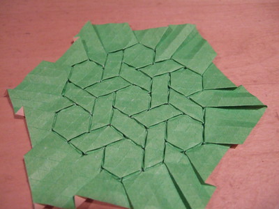
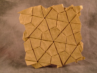
(click for the original image)
Known techniques
The most popular technique in flagstone tessellation is probably the one proposed by Eric Gjerde in his book Origami Tessellations 1.
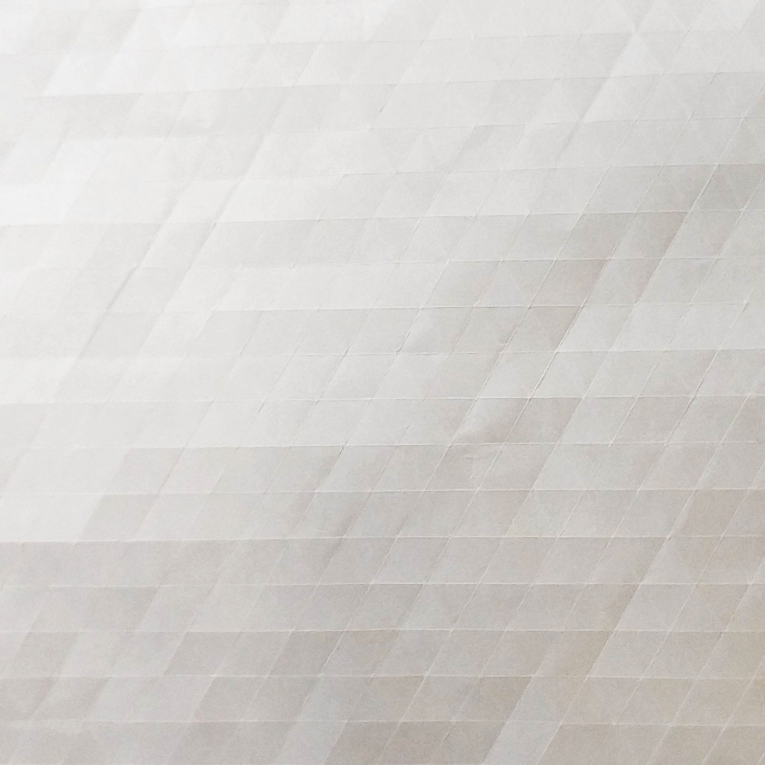
This technique consists in pre-creasing our sheet according to a square or triangular grid.
After that we start to explore possible patterns for flagstone tessellations by folding along the pre-creases made at the beginning.
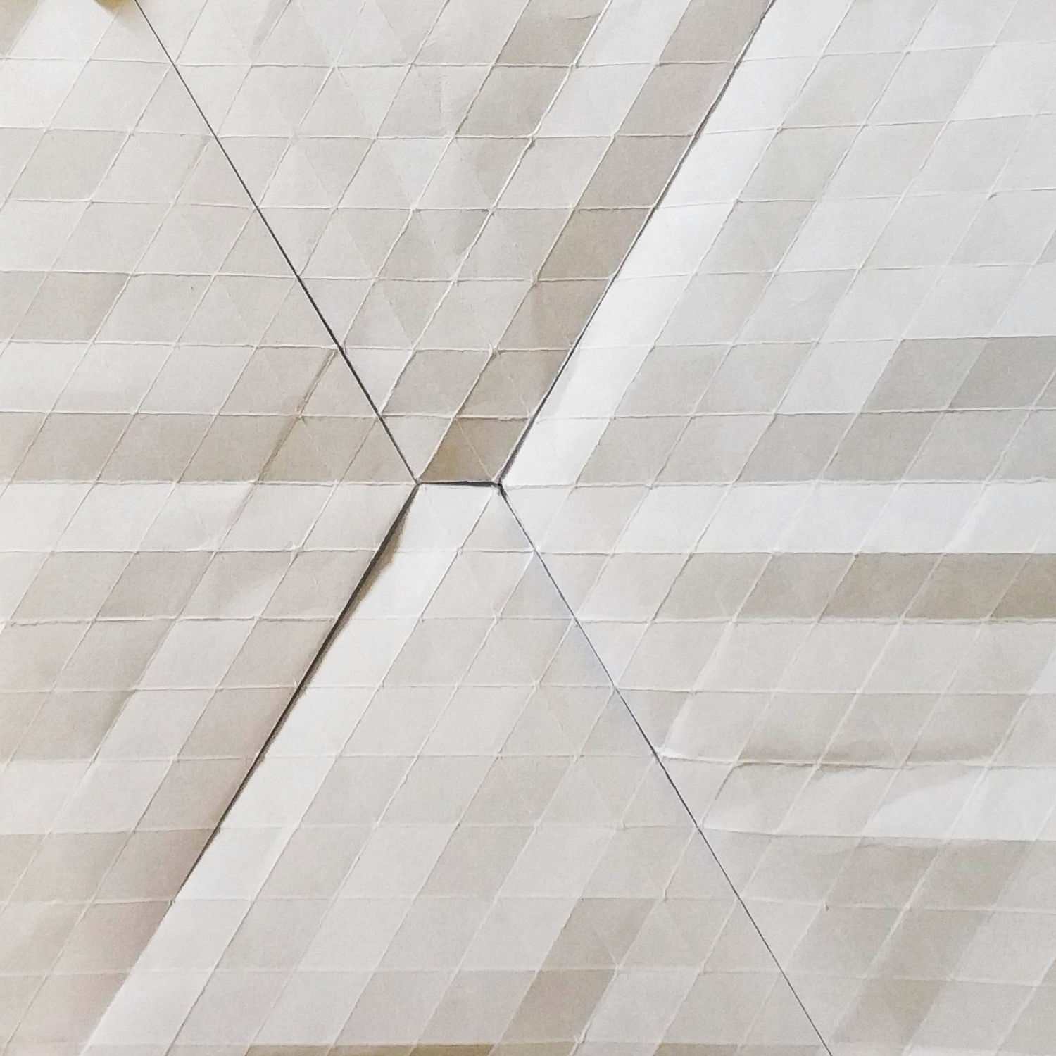
In fig.2 there is an example of pre-creased sheet, and a flagstone tessellation obtained from that sheet.
The explanation and illustration of this technique would be too long to be covered here and goes beyond the scope of the article.
Therefore, I suggest you follow the book mentioned above, Origami Tessellations, containing the detailed and visual explanation of various tessellation techniques,
as well as commented illustrations, step by step, for the realization of multiple models from a pre-creased sheet according to grids.
A more general technique is the geometric construction proposed by Robert J. Lang in his book Twists, Tilings and Tessellations 2.
Lang dedicates several pages to Flagstone tessellations, starting from the mathematical conditions necessary for a flagstone tessellation to be feasible and foldable,
then providing a geometric algorithm for the construction of a generic tessellation node.
Below is illustrated a possible geometric construction using a modified version of this algorithm, which simplifies its application.
Molecules and geometric construction
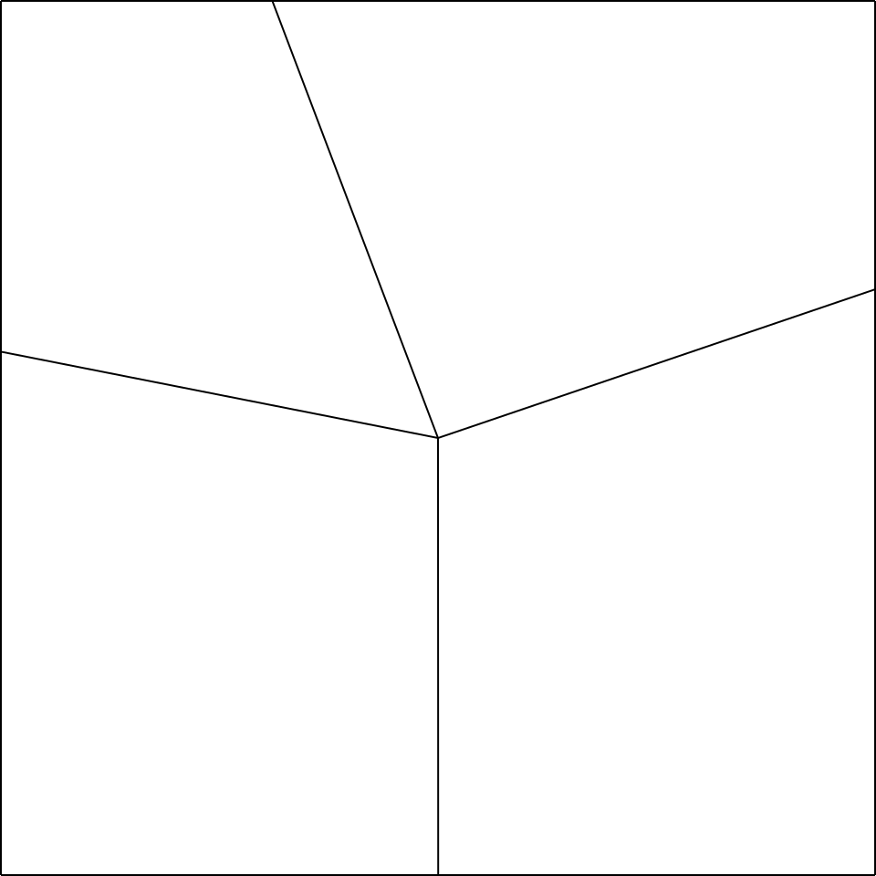
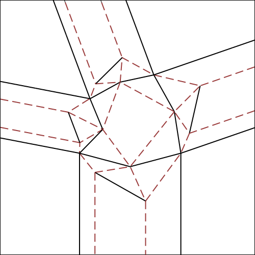
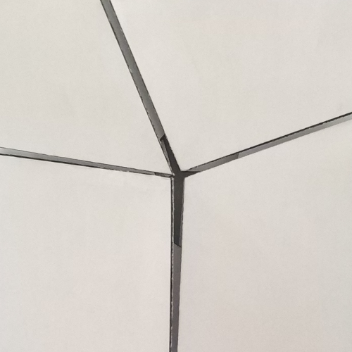
Let’s consider any node of a finished tessellation model (fig.3a); the part corresponding to the node, in the initial crease pattern (fig.3b e 3c) is commonly called tessellation molecule.


The rectangles of paper, instead, corresponding to the lines that form the node, will be called “strips” of the node.
Now, let’s first see how to determine these rectangular paper strips between the polygons, and then move on to the construction of the relative molecule.
Strips contruction
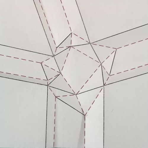
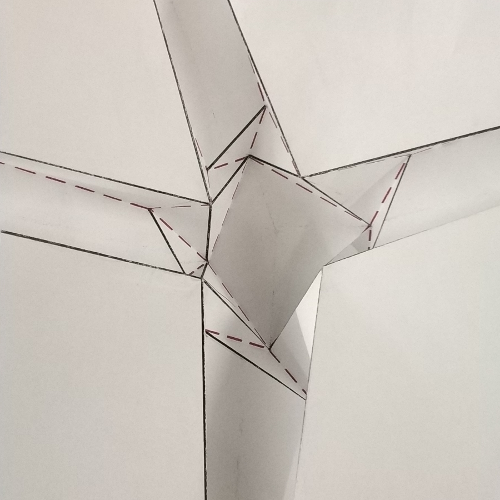
So, let’s start by saying that the “strips” of paper between the polygons, constitute the excess of paper that, when folded, allows us to join the edges of the adjacent polygons, to form the final node with flagstone effect (vedi fig.4).
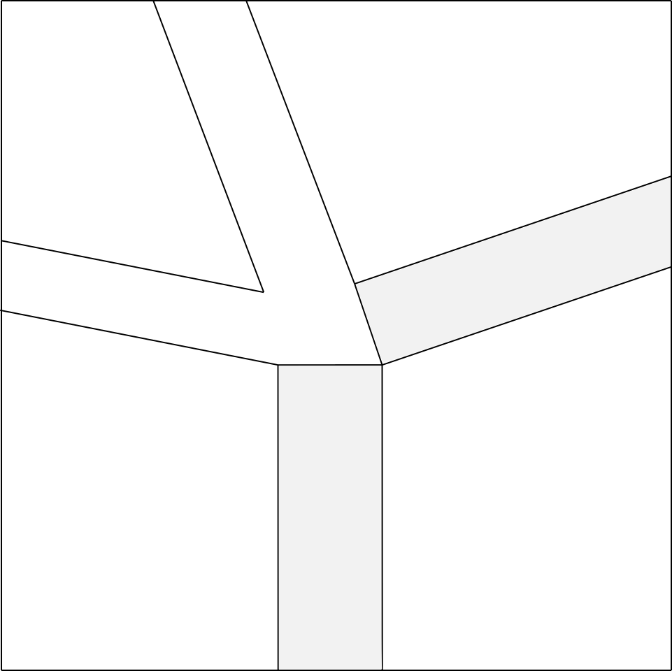
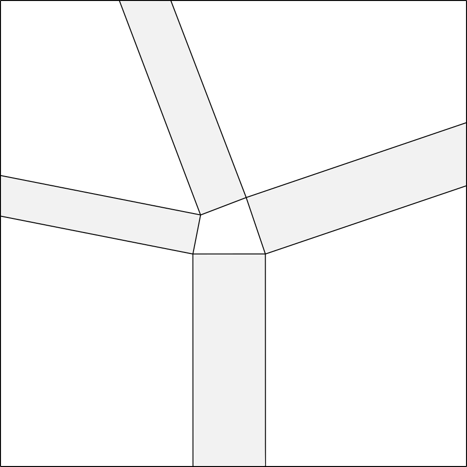
Having said that, let’s start from the node you want to make (i.e. the node in fig.5a).
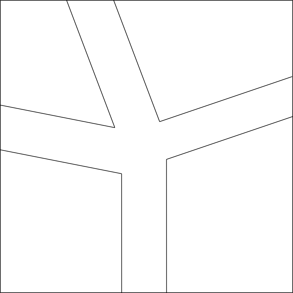
Let’s imagine opening the node mentioned (fig.5b), and we add a rectangle of small width at will 3
between the two polygons below, and a rectangle between the two polygons on the right (fig.5c).
At this point, the remaining two rectangles that we have to add will have a compulsory width, determined by their joining point, which will be the vertex of the polygon on the top left, as shown in fig.5d.
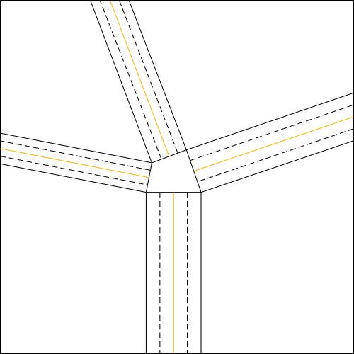
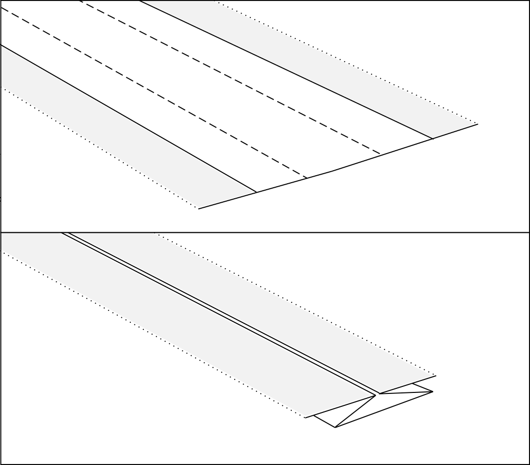
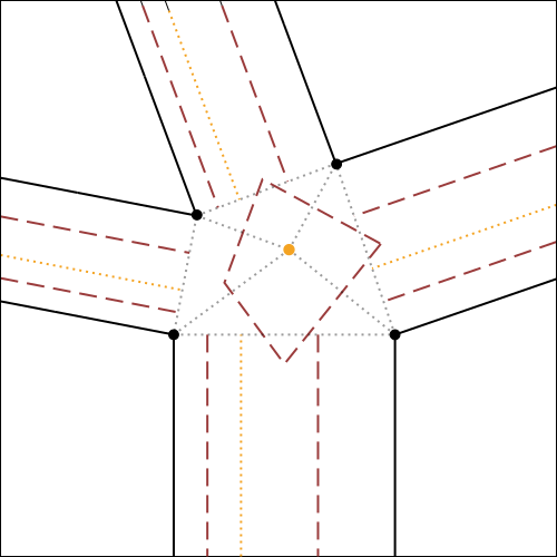
Once determined the strips of the node, we draw the two lines inside each strip, parallel to the long sides of the same, necessary to make the double pleat (fig.4).
According to the position in which we want to make the double pleat converge, the two lines will be chosen at a specific distance from the parallel sides of the strip;
in particular, they will be chosen at a distance that is halfway between the convergence line (orange lines in fig.6) and the relative parallel side.
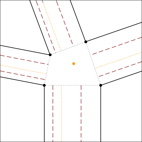
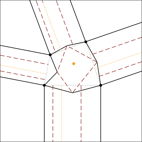
The next step is to determine the molecule delimited by these strips.
Molecule construction
In fig.7, the algorithm for the construction of molecule 4 is illustrated and explained exhaustively, using as initial reference the crease pattern of fig.6.
It is possible to click on each step to zoom on it.
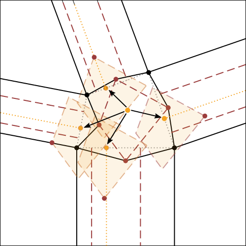

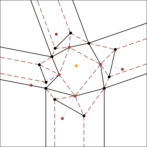
This algorithm is suitable for use in vector drawing software (e.g. Inkscape), while it is more complicated to use directly on paper. The following image (fig.8) shows a practical example of the use of such algorithm.
Analytical calculation
Starting from the final valid crease pattern of a molecule, we can use analytic geometry to calculate the values of the points of interest and segments of the crease pattern, based on the initial known data.
Let’s analyze below the case of a molecule with 4 branches (4 strips).
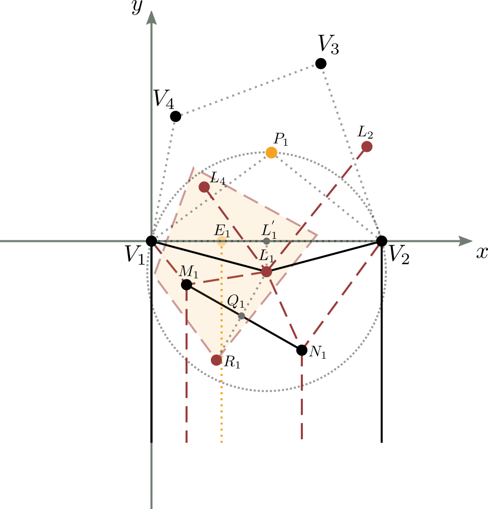
Let’s consider figure 9 in which a complete and valid crease pattern of a molecule is reported on the Cartesian plane,
with the first vertex of the central part corresponding to the center of the axes of the plane, and the base of the central part lying on the x-axis.
The initial known data are essentially the shape and size of the central part of the molecule (the quadrilateral $V_1V_2V_3V_4$ in the figure),
defined completely by 3 of its corners and 2 of its sides, the position of the center $P_1$ within the central part, and the $E_i$ convergence point of the double pleat for each strip $i$, with $1 \leq i \leq 4$.
Therefore, let’s use, for convenience:
$\hat{V_4V_1V_2} = \alpha_1$, $\quad\hat{V_1V_2V_3} = \alpha_2$, $\quad\hat{V_2V_3V_4} = \alpha_3$
$\overline{V_1V_2} = \ell_1$, $\quad\overline{V_2V_3} = \ell_2$, \(\quad P_1(P_{1x}, P_{1y})\)
$\overline{V_1E_1}=c_1$, $\quad \overline{V_2E_2}=c_2$, $\quad \overline{V_3E_3}=c_3$, $\quad \overline{V_4E_4}=c_4$
with $\alpha_1$, $\alpha_2$, $\alpha_3$, $\ell_1$, $\ell_2$, \(P_{1x}\), \(P_{1y}\) e $c_1$, $c_2$, $c_3$, $c_4$ known.
The values $\alpha_1$, $\alpha_2$ e $\alpha_3$ are linked to the fact that $V_1V_2V_3V_4$ is a convex quadrilateral.
$\ell_1$ e $\ell_2$ are greater than zero.
$P_{1x}$ e $P_{1y}$ are bound by the fact that the point $P_1$ is inside the quadrilateral $V_1V_2V_3V_4$.
The values $c_1$, $c_2$, $c_3$ e $c_4$ are positive, are positive, between 0 and the width of the relative strips.

If you look at the image, you can see that in order to draw the crease pattern univocally, it is necessary to know the position of the $L_i$, $M_i$ ed $N_i$ points of each strip $i$, with $1\le i \le 4$. Let’s start by calculating the values of points $P_1$, $M_1$ e $N_1$ of the first strip.
Calculation of values of the first strip
Let’s use the following image (fig.10), which is an enlargement of figure 9, centered only on the first strip, extended with all the intermediate steps of the geometric construction of figure 7.
Having chosen, for convenience, the point $V_1$ matching the origin of the axes and the segment $\overline{V_1V_2}$ lying on the $x$-axis, it follows that the coordinates of points $V_1$ and $V_2$ are:
$V_1(0,0)$ e $V_2(\ell_1,0)$
Now, from the geometry of the triangle we know that the point of intersection of the axes of the sides of any triangle coincides with the circumcenter,
that is, with the center of the circumference circumscribed to that triangle.
Since the segments $\overline{L_{4}L_{1}}$ and $\overline{L_{1}L_{2}}$ are the axes of the segments $\overline{P_1V_1}$ and $\overline{P_1V_2}$,
then the point $L_1$ is the circumcenter of the triangle $\overset{\Delta}{V_1V_2P_1}$.
So, the $x$-axis of point $L_1$, being the axis of segment $\overline{V_1V_2}$ passing through $L_1$, is $\displaystyle L_{1x} = \frac{\overline{V_1V_2}}{2} = \frac{\ell_1}{2}$.
To calculate the ordinate of point $L_1$ instead, we can consider the fact that $\overline{V_1L_1}$, $\overline{V_2L_1}$ and $\overline{P_1L_1}$ are radii of the circumference circumscribed to triangle $\overset\Delta{V_1V_2P_1}$;
in particular, we have $\overline{V_1L_1}=\overline{P_1L_1}$.
Therefore, placing $\overline{L_1^{‘}L_1} = L_{1y} = y$, we have:
then
\[\displaystyle L_1\left(\frac{\ell_1}{2}, \frac{P_{1x}^2-P_{1x}\cdot \ell_1 + P_{1y}^2}{2\cdot P_{1y}} \right)\]Let’s now calculate $R_1$.
Being, by construction, $\overline{L_1R_1} = \overline{P_1E_1}$, then:
which is
\[\displaystyle R_1\left(\frac{\ell_1}{2} - P_{1x} + c_1, \frac{P_{1y}^2+P_{1x}\cdot \ell_1 -P_{1x}^2}{2\cdot P_{1y}} \right)\]Let’s calculate $Q_1$.
Being $Q_1$, by construction, the midpoint of $\overline{L_1R_1}$, we have:
which is
\[Q_1\left(\frac{\ell_1-P_{1x}+c_1}{2}, \frac{P_{1x}^2-P_{1x}\cdot \ell_1}{2\cdot P_{1y}} \right)\]Let’s now calculate $M_1$ and $N_1$, referring to figure 11 below.
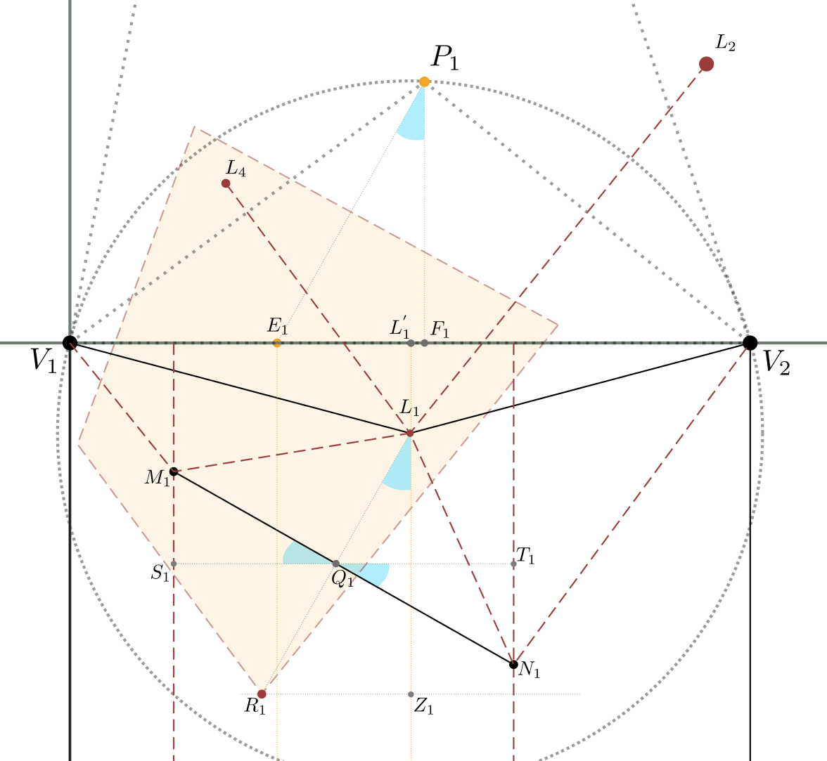
Let’s consider the $\overline{S_1Q_1}$ segment perpendicular to $\overline{L_1Z_1}$ and parallel to $\overline{V_1V_2}$.
Being also, for the initial construction, $\overline{M_1N_1}$ perpendicular to $\overline{L_1R_1}$, and $\overline{L_1R_1} = \overline{P_1E_1}$,
we can see that the angles in blue marked in the image are all the same; that is
Let’s now calculate $M_1$.
The $x$-axis of $M_1$ è già nota per costruzione e vale $\displaystyle M_{1x} = \frac{\overline{V_1E_1}}{2} = \frac{c_1}{2}$ .
The ordinate instead is given by:
Since, as seen above, $ \small\hat{S_1Q_1M_1} = \small\hat{E_1P_1F_1}$, by substituting you have:
\[M_{1y} = Q_{1y} + \overline{S_1Q_1}\cdot \tan(\small\hat{E_1P_1F_1}) = Q_{1y} + \overline{S_1Q_1}\cdot \frac{\overline{E_1F_1}}{\overline{P_1F_1}} = \\ = Q_{1y} + (Q_{1x}-M_{1x})\cdot \frac{P_{1x}-E_{1x}}{P_{1y}} = Q_{1y} + (Q_{1x}-M_{1x})\cdot \frac{P_{1x}-c_1}{P_{1y}}\]Finally, replacing the values $Q_{1x}$, $Q_{1y}$ and $M_{1x}$ ound previously, we have:
\[M_{1y} = \frac{P_{1x}^2-P_{1x}\cdot \ell_1}{2\cdot P_{1y}} + \left(\frac{\ell_1-P_{1x}+c_1}{2}-\frac{c_1}{2}\right)\cdot \frac{P_{1x}-c_1}{P_{1y}}\]then
\[M_1\left(\frac{c_1}{2}, \frac{P_{1x}^2-P_{1x}\cdot \ell_1}{2\cdot P_{1y}} + \left(\frac{\ell_1-P_{1x}}{2}\right)\cdot \frac{P_{1x}-c_1}{P_{1y}} \right)\]Finally, let’s calculate $N_1$, using a similar reasoning as for $M_1$.
The $x$-axis of $N_1$ is $\displaystyle N_{1x} = \frac{E_{1x}+V_{2x}}{2} = \frac{c_1+\ell_1}{2}$ .
The $y$-axis instead, is given by:
Since, as seen above, $ \small\hat{T_1Q_1N_1} = \small\hat{E_1P_1F_1}$, by substituting we have:
\[N_{1y} = Q_{1y} - \overline{Q_1T_1}\cdot \tan(\small\hat{E_1P_1F_1}) = Q_{1y} - \overline{Q_1T_1}\cdot \frac{\overline{E_1F_1}}{\overline{P_1F_1}} = \\ = Q_{1y} - (N_{1x}-Q_{1x})\cdot \frac{P_{1x}-E_{1x}}{P_{1y}} = Q_{1y} - (N_{1x}-Q_{1x})\cdot \frac{P_{1x}-c_1}{P_{1y}}\]Finally, replacing the values $Q_{1x}$, $Q_{1y}$ and $N_{1x}$ found previously, we have:
\[N_{1y} = \frac{P_{1x}^2-P_{1x}\cdot \ell_1}{2\cdot P_{1y}} - \left(\frac{c_1+\ell_1}{2}-\frac{\ell_1-P_{1x}+c_1}{2}\right)\cdot \frac{P_{1x}-c_1}{P_{1y}}\]which is
\[N_1\left(\frac{c_1+\ell_1}{2}, \frac{P_{1x}^2-P_{1x}\cdot \ell_1}{2\cdot P_{1y}} - \frac{P_{1x}}{2}\cdot \frac{P_{1x}-c_1}{P_{1y}} \right)\]So, to summarize, the points of interest for the construction of the crease pattern, relative to the first strip (side $\overline{V_1V_2}$ side of the quadrilateral) are:
\[\begin{equation}\begin{cases} \displaystyle L_1\left(\enspace\frac{\ell_1}{2},\enspace\frac{P_{1x}^2-P_{1x}\cdot \ell_1 + P_{1y}^2}{2\cdot P_{1y}}\enspace \right) \\ \displaystyle M_1\left(\enspace\frac{c_1}{2}\enspace,\enspace\frac{P_{1x}^2-P_{1x}\cdot \ell_1}{2\cdot P_{1y}} + \left(\frac{\ell_1-P_{1x}}{2}\right)\cdot \frac{P_{1x}-c_1}{P_{1y}}\enspace \right) \\ \displaystyle N_1\left(\enspace\frac{c_1+\ell_1}{2}\enspace,\enspace\frac{P_{1x}^2-P_{1x}\cdot \ell_1}{2\cdot P_{1y}} - \frac{P_{1x}}{2} \cdot \frac{P_{1x}-c_1}{P_{1y}}\enspace \right) \end{cases}\end{equation}\label{a}\tag{1}\]Calculation of the second strip values
To calculate the values $L_2$, $M_2$ and $N_2$ of the second strip (the one on the $\overline{V_2V_3}$ side), we can imagine to translate and rotate the molecule in such a way that the point $V_2$ coincides with the origin of the axes and the segment $\overline{V_2V_3}$ is placed on the $x$-axis (figure 12 5).
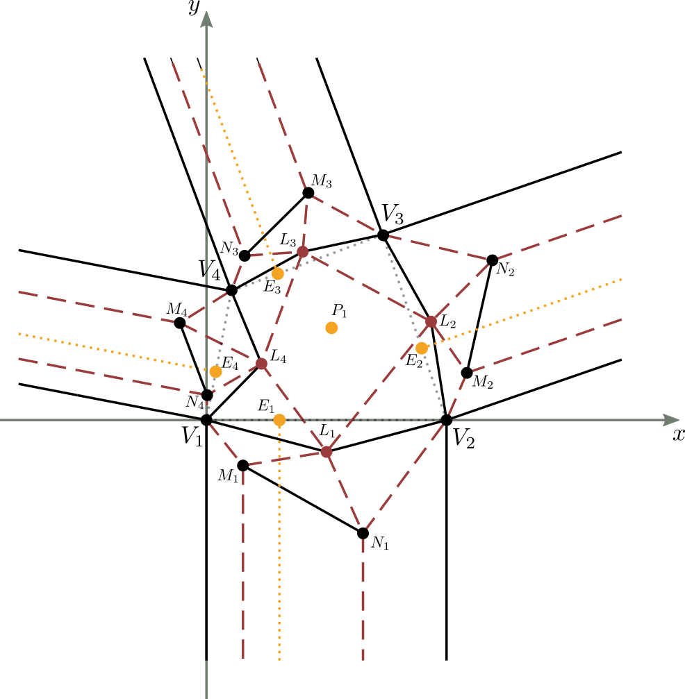
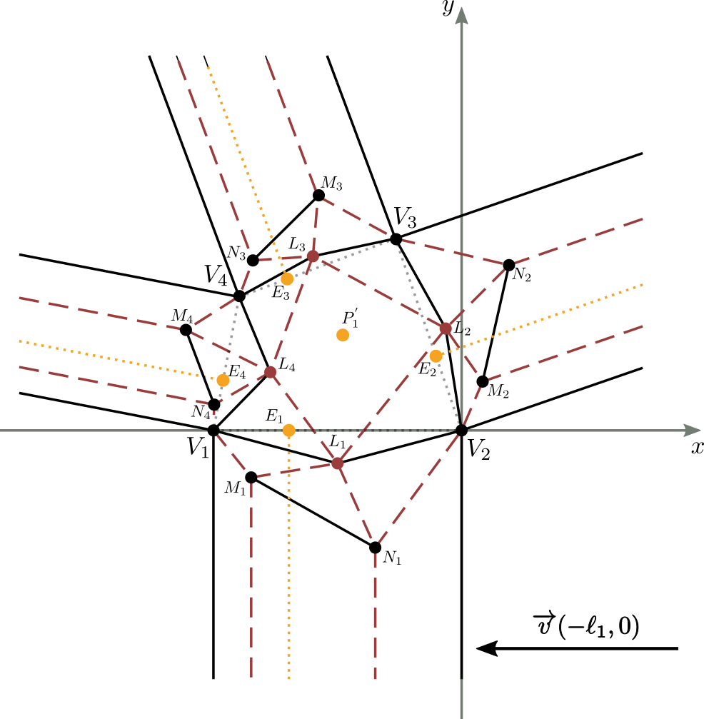
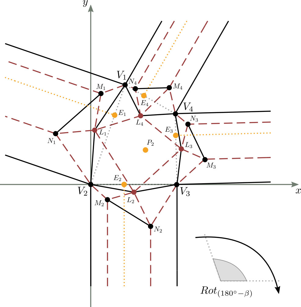
Figure 12b shows the result of the translation of the molecule in figure 12a, by the vector $\overrightarrow{v}(-\ell_1,0)$. The equations of this translation have the following values:
\[T_{\overrightarrow{v}} \quad \begin{cases} x^{'} = x -\ell_1 \\ y^{'} = y \end{cases}\]where $x$ and $y$ are the known coordinates of a point in the plane, while $x^{‘}$ and $y^{‘}$ are the coordinates of its transformation, following the translation.
Specifically, we calculate the coordinates of the point $P^{‘}_1$, transformed of $P_1$ according to the said translation. We have:
which is \(P^{'}_1(P_{1x} -\ell_1, P_{1y})\).
We then apply to image 12b a clockwise rotation around the origin, of amplitude equal to $180^{\circ} - \alpha_2$, in order to have $\overline{V_2V_3}$ lying on $x$ axis. We have:
\[Rot_{(180^{\circ} -\alpha_2)} \quad \begin{cases} x^{'} = x\cos{(180^{\circ} -\alpha_2)} + y \sin{(180^{\circ} -\alpha_2)} \\ y^{'} = -x\sin{(180^{\circ} -\alpha_2)} + y \cos{(180^{\circ} -\alpha_2)} \end{cases}\]where $x$ e $y$ are the known coordinates of a point in the plane, while $x^{‘}$ e $y^{‘}$ are the coordinates of its transformation, following rotation.
Specifically, we calculate the coordinates of the point $P_2$, transformed by $P^{‘}_1$ according to the above rotation. We have:
which is \(P_2(\enspace(\ell_1-P_{1x})\cdot\cos{\alpha_2} + P_{1y}\cdot\sin{\alpha_2}\enspace,\enspace(\ell_1-P_{1x})\cdot\sin{\alpha_2} - P_{1y}\cdot\cos{\alpha_2}\enspace)\)
At this stage, we can proceed to the calculation of $L_2$, $M_2$ and $N_2$ values (figure 12c), using the same formulas obtained for the first strip (previous sub-paragraph).
Let’s then start from figure 12c, result of the transformations analyzed above.
The initial known data are always the same that we defined at the beginning of this paragraph,
except for the coordinates of point $P_1$, which have been transformed in point $P_2$,
following the two operations of translation and rotation.
Therefore, we have the following data:
$\quad\hat{V_1V_2V_3} = \alpha_2$
$\quad\overline{V_2V_3} = \ell_2$
\(\quad P_2(\enspace(\ell_1-P_{1x})\cdot\cos{\alpha_2} + P_{1y}\cdot\sin{\alpha_2}\enspace,\enspace(\ell_1-P_{1x})\cdot\sin{\alpha_2} - P_{1y}\cdot\cos{\alpha_2}\enspace)\)
$\quad \overline{V_2E_2}=c_2$
where $\alpha_2$, $\ell_2$, \(P_{2x}\), \(P_{2y}\) and $c_2$ are known.
If we replace $\ell_1$ with $\ell_2$, $c_1$ with $c_2$, and the values of $P_1$ with those of $P_2$ in formulae of $\eqref{a}$, we get the desired $L_2$, $M_2$ and $N_2$ values. We have:
\[\begin{equation}\begin{cases} \displaystyle L_2\left(\frac{\ell_2}{2}, \frac{(P_{2x})^2-P_{2x}\cdot \ell_2 + (P_{2y})^2}{2\cdot P_{2y}} \right) \\ \displaystyle M_2\left(\frac{c_2}{2}, \frac{(P_{2x})^2-P_{2x}\cdot \ell_2}{2\cdot P_{2y}} + \left(\frac{\ell_2-P_{2x}}{2}\right)\cdot \frac{P_{2x}-c_2}{P_{2y}} \right) \\ \displaystyle N_2\left(\frac{c_2+\ell_2}{2}, \frac{(P_{2x})^2-P_{2x}\cdot \ell_2}{2\cdot P_{2y}} - \frac{P_{2x}}{2} \cdot \frac{P_{2x}-c_2}{P_{2y}} \right) \end{cases}\end{equation}\label{b3}\tag{2.3}\]where \(P_2(\enspace(\ell_1-P_{1x})\cdot\cos{\alpha_2} + P_{1y}\cdot\sin{\alpha_2}\enspace,\enspace(\ell_1-P_{1x})\cdot\sin{\alpha_2} - P_{1y}\cdot\cos{\alpha_2}\enspace)\).
Calculation of n-th strip values (generalization)
We can recursively apply the transformations used in the calculation of the values for the second strip, to determine the values of a generic strip $n$.
Therefore, we generalize by calculating the $L_n$, $M_n$ and $N_n$ values of the $n$-th strip.
Let us consider figure 13a, which represents a generic molecule, and in particular its strip ($n$-1)-th ed $n$-th.
Let’s then apply a new translation and rotation to this molecule so that the point $V_n$ coincides with the origin of the axes (point $V_{n-1}$) and the segment $\overline{V_nV_{n+1}}$ lies on the $x$-axis (figure 13c).
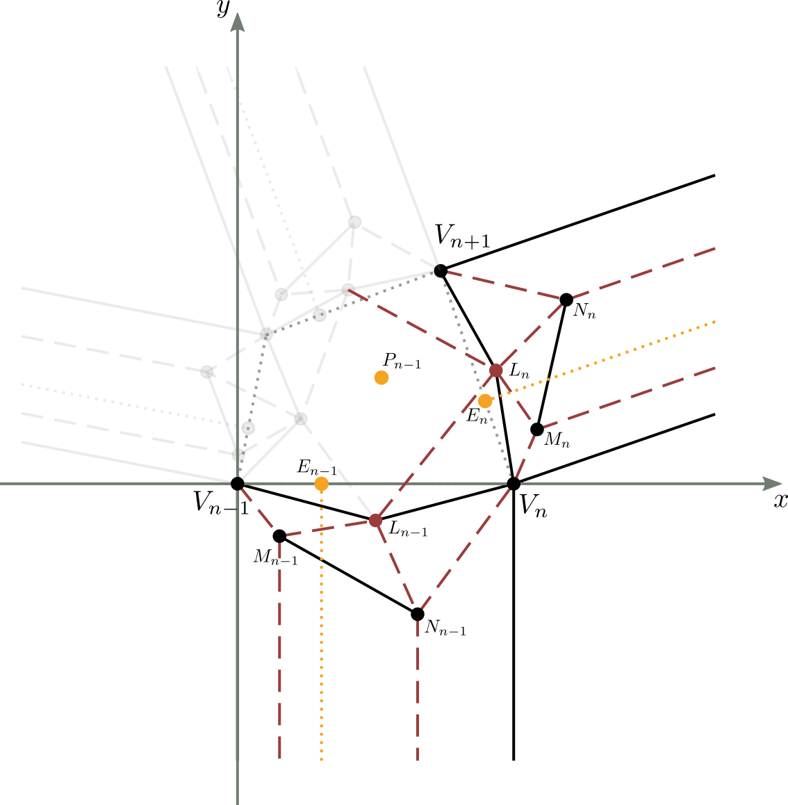

For the translation of figure 13b we have (similarly to what already seen for the second strip):
\[T_{\overrightarrow{v}} \quad \begin{cases} x^{'} = x -\ell_{n-1} \\ y^{'} = y \end{cases}\]where $x$ and $y$ are the known coordinates of a point in the plane, while $x^{‘}$ and $y^{‘}$ are the coordinates of its transformation, following the translation.
Specifically, we calculate the coordinates of the point \(P^{'}_{n-1}\), transformed of $P_{n-1}$ according to the above translation. We have:
which is \(P^{'}_{n-1}(\enspace P_{n-1_{x}} -\ell_{n-1} \enspace,\enspace P_{n-1_{y}} \enspace)\).
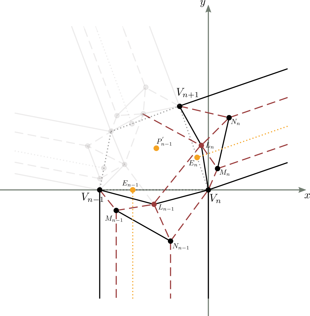
We then apply to figure 13b a clockwise rotation around the origin, with an amplitude equal to $180^{\circ} - \alpha_n$, al fine di avere $\overline{V_nV_{n+1}}$ giacente sull’asse $x$. Si ha:
\[Rot_{(180^{\circ} -\alpha_n)} \quad \begin{cases} x^{'} = x\cos{(180^{\circ} -\alpha_n)} + y \sin{(180^{\circ} -\alpha_n)} \\ y^{'} = -x\sin{(180^{\circ} -\alpha_n)} + y \cos{(180^{\circ} -\alpha_n)} \end{cases}\]where $x$ and $y$ are the known coordinates of a point in the plane, while $x^{‘}$ and $y^{‘}$ are the coordinates of its transformation, following rotation.
$\alpha_n$ is the angle of the central polygon, of vertex $V_n$.
Specifically, we calculate the coordinates of the point \(P_n\), transformed of $P^{‘}_{n-1}$ according to the above rotation. We have:
Replacing values of \(P^{'}_{n-1x}\) e \(P^{'}_{n-1y}\) obtained from $\eqref{c1}$ we have:
\[\begin{equation}P_n \rightarrow \begin{cases} P_{nx} = (\ell_{n-1}-P_{n-1_{x}})\cdot\cos{\alpha_n} + P_{n-1y}\cdot\sin{\alpha_n} \\ P_{ny} = (\ell_{n-1}-P_{n-1_{x}}) \cdot\sin{\alpha_n} - P_{n-1y}\cdot\cos{\alpha_n} \end{cases} \end{equation}\label{c2}\tag{3.2}\]which is \(P_n(\enspace (\ell_{n-1}-P_{n-1_{x}})\cdot\cos{\alpha_n} + P_{n-1y}\cdot\sin{\alpha_n} \enspace,\enspace (\ell_{n-1}-P_{n-1_{x}}) \cdot\sin{\alpha_n} - P_{n-1y}\cdot\cos{\alpha_n} \enspace)\).
We therefore proceed to calculate the $L_n$, $M_n$ e $N_n$, values, always using the formulas of $\eqref{a}$.
Let’s start from figure 13c, result of the transformations analyzed above.
The initial known data, in function of $n$, are:
$\widehat{V_{n-1}V_nV_{n+1}} = \alpha_n$
$\overline{V_nV_{n+1}} = \ell_n$
\(P_n(\enspace (\ell_{n-1}-P_{n-1_{x}})\cdot\cos{\alpha_n} + P_{n-1y}\cdot\sin{\alpha_n} \enspace,\enspace (\ell_{n-1}-P_{n-1_{x}}) \cdot\sin{\alpha_n} - P_{n-1y}\cdot\cos{\alpha_n} \enspace)\)
$\overline{V_nE_n}=c_n$
where $\alpha_n$, $\ell_n$, \(P_{nx}\), \(P_{ny}\) and $c_n$ are known.
If we replace $\ell_1$ with $\ell_n$, $c_1$ with $c_n$, and the $P$ values with those of $P_n$ in formulae of $\eqref{a}$, we get the desired $L_n$, $M_n$ e $N_n$ values. We have:
\[\begin{equation}\begin{cases} \displaystyle L_n\left(\frac{\ell_n}{2}, \frac{(P_{nx})^2-P_{nx}\cdot \ell_n + (P_{ny})^2}{2\cdot P_{ny}} \right) \\ \displaystyle M_n\left(\frac{c_n}{2}, \frac{(P_{nx})^2-P_{nx}\cdot \ell_n}{2\cdot P_{ny}} + \left(\frac{\ell_n-P_{nx}}{2}\right)\cdot \frac{P_{nx}-c_n}{P_{ny}} \right) \\ \displaystyle N_n\left(\frac{c_n+\ell_n}{2}, \frac{(P_{nx})^2-P_{nx}\cdot \ell_n}{2\cdot P_{ny}} - \frac{P_{nx}}{2} \cdot \frac{P_{nx}-c_n}{P_{ny}} \right) \end{cases}\end{equation}\label{c3}\tag{3.3}\]where \(P_n(\enspace (\ell_{n-1}-P_{n-1_{x}})\cdot\cos{\alpha_n} + P_{n-1y}\cdot\sin{\alpha_n} \enspace,\enspace (\ell_{n-1}-P_{n-1_{x}}) \cdot\sin{\alpha_n} - P_{n-1y}\cdot\cos{\alpha_n} \enspace)\).
Conclusions
We have therefore shown how to construct geometrically, and how to analytically calculate generic flagstone molecules (with $n$ branches), to make tessellations of varying complexity.
Specifically, the geometric construction is particularly useful for the computer design of the molecule, using vector graphics software such as Inkscape.
The analytical calculation, for its part, provides us with the exact formulas that allow us to switch from the initial known data to the final values of the molecule;
this has been fundamental for the realization of a software of calculation/simulation of flagstone molecules with $n$ branches, where by entering the desired initial data,
we obtain in real time the crease pattern of the specific molecule, with the possibility to save it in vector format (SVG).
This software is described in this article and is available on Github
-
Eric Gjerde, Origami Tessellations, CRC Press, 2008. ↩
-
Robert J. Lang, Twists, Tilings, And Tessellations, CRC Press, 2017. ↩
-
This is the width of the paper strips: the narrower the strips, the smaller the relative molecules will be and the less paper will be used in general for tessellation; on the other hand, the more difficult it will be to fold them. ↩
-
This algorithm is a modified version of the algorithm proposed by R.J.Lang in his book “Twists, Tilings, and Tessellations”, (pp.449). ↩
-
With the exception of point $P_1$, which is translated into $P^{‘}_1$, and then rotated into $P_2$, for convenience, the other points in the plane are left unchanged in their labels ↩